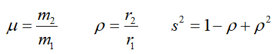
A Klemperer rosette is a system of an equal number of two kinds of bodies arranged in a regular alternating pattern around the center of mass.
These systems were first described by Klemperer in 1962.
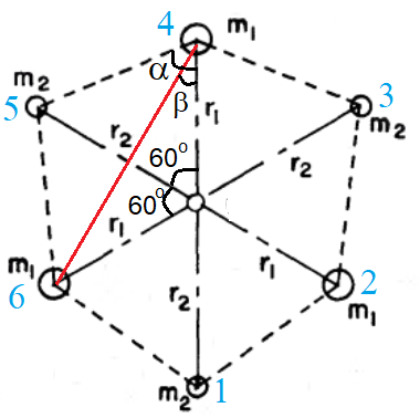
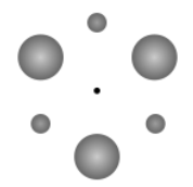
The figure below shows a hexagonal rosette. The distances of the two kinds of bodies from the center are in general different.
Klemperer also described rhombic and octagonal rosettes.
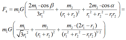
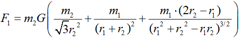
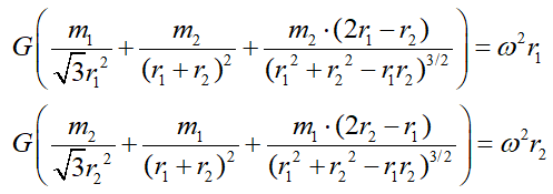
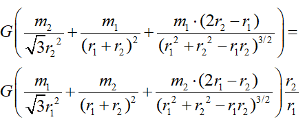
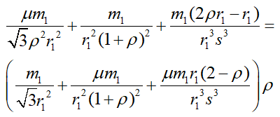
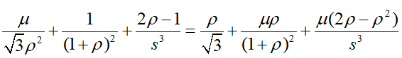
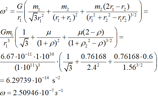
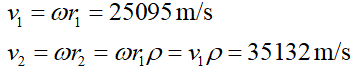
To construct this simulation we have used some rather complicated formulas to calculate the velocities of the bodies after choosing their distances from the center of the polygon
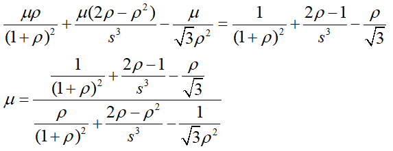
and the mass of the lightest bodies (1, 3 and 5). The mass of bodies 2, 4 and 6 must then have a particular value, as shown in the right column.
The parameters are calculated to high precision.
Exercise
-
Start the simulation. The orbits seem stable at first, but what happens after a while?
To make the orbits stable for many revolutions, the initial positions and velocities must have even higher precision.
All rosettes are unstable. Any deviation along a tangent from the "correct" position brings a body closer to one neighbor and further from another. Then the gravitational force becomes greater for the closer neighbor and less for the farther neighbor, pulling the perturbed body further towards its closer neighbor and amplifying the deviation rather than reducing it. An inward radial deviation causes the perturbed body to get closer to all other bodies, increasing the force on the body and increasing its orbital velocity, which leads indirectly to a tangential deviation. -
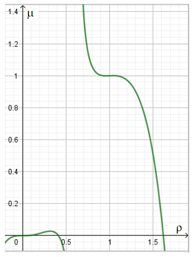
Looking at the graph in the right column, it is apparent that there exists another possible domain for
μ less than 0.41. The maximum of μ is 0.31891 for ρ = 0.02801.
Construct a simulation using these values.